Overview of Probability
Probability provides the means to analyze the possible outcomes of a given process.
Specifically, probability is concerned with defining the frequency of each possible outcome in relation to the range and distribution of all possible outcomes.
The range and distribution of all possible outcomes for a process is referred to as the probability distribution of that process. The following are discussions of commonly seen distribution types:
Uniform Distribution
Consider the roll of a single die as a process. There are six possible outcomes (1, 2, 3, 4, 5, or 6), each of which is equally likely. As a result, we can say that each outcome has one chance in six of occurring.
Certainty is defined as 1.0 (or 100 percent). If you divide 1.0 by the six possible outcomes, you can see that each result in this case has a probability of 0.167. You can then construct the following table to represent all the possible outcomes and their probabilities:
| Outcome | Probability |
|---|---|
| 1 | 0.167 |
| 2 | 0.167 |
| 3 | 0.167 |
| 4 | 0.167 |
| 5 | 0.167 |
| 6 | 0.167 |
We can also chart this distribution of probability using x and y coordinates, where x represents the range of outcomes and y represents the probability of each outcome:
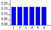
Because the probabilities for all the possible outcomes are the same in this case, this type of distribution is called a uniform distribution.
Triangular Distribution
Consider the combined score from rolling a pair of dice. The range of possible outcomes is from two to twelve. Yet, as any gambler knows, these outcomes are not equally likely. Rolling a twelve is much less likely than rolling a seven because there are many ways of achieving a seven but only one way to roll a twelve.
If we represent this distribution as a table, we get the following:
| Outcome | Probability |
|---|---|
| 2 | 0.028 |
| 3 | 0.056 |
| 4 | 0.085 |
| 5 | 0.111 |
| 6 | 0.139 |
| 7 | 0.167 |
| 8 | 0.139 |
| 9 | 0.111 |
| 10 | 0.085 |
| 11 | 0.056 |
| 12 | 0.028 |
Because the height of the triangle above any point along the x-axis represents the probability of the outcome represented by that point, the illustration shows clearly how much more probable it is to roll a seven than to roll any other number.
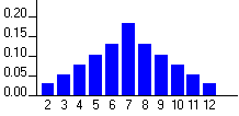
In this example, a symmetrical triangle is produced in which the probability declines from the apex at the same rate in both directions.
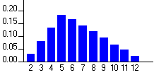
Not all triangular distributions are symmetrical. Given other circumstances, it would be possible to have a triangular distribution such as this:
Normal Distribution
Just as rolling a pair of dice adds complexity to the possible outcomes of the process when compared to rolling a single die, adding more and more dice increases the number of possible outcomes. Eventually, if we reach a level of sufficient complexity, the probability distribution looks something like this:
This distribution is called a normal distribution, and it turns out that the sum of the outcomes of multiple tries of any random process tends towards this curve.
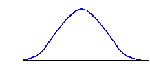
The normal distribution is an example of a continuous distribution. Unlike the examples of the uniform and triangular distributions in which each possible outcome was discrete, the curved shape of the normal distribution depicts a range of continuous rather than discrete outcomes. As a result, it is the area under the curve between any two x values that represents the probability of the outcome falling between these two values.
Both uniform and triangular distributions can represent continuous outcomes as well.
Beta Distribution
Depending on how the distribution is defined, there are a number of ways of representing asymmetrical probability. However, for the purposes of Open Plan, a family of distributions known as beta distributions is used.
The beta distribution, like the triangular distribution, is primarily used to describe asymmetrical probability. However, a beta distribution differs from triangular distribution because its shape effectively precludes outcomes at the extremes of the distribution from having any significant probability. By contrast, a triangular distribution allows for a significant probability for outcomes at the extreme limits of the range, no matter how much the distribution is skewed.